7. SciPy最小二乘法

最小二乘法则是一种统计学习优化技术，它的目标是最小化误差平方之和来作为目标$J(\theta)$，从而找到最优模型。

$$ J(\theta) = \min\sum_{i = 1}^m (f(x_i) - y_i)^2 $$ 其中，$f(x_i) = a_0 + a_1x^1+a_2x^2+\dots+a^nx^n$即是要找到的模型，而$y_i$是已有的观测值。 SciPy的linalg下的lstsq只需给出方程$f(x_i)$的模型即A以及样本$y_i$便可求得方程的各个系数。

7.1 线性最小二乘法

假设真实的模型是$y = 2 x + 1$，我们有一组数据($x_i,y_i$)共100个，看能否基于这100个数据找出$x_i$和$y_i$的线性关系方程$y = 2 x + 1$？我们可以通过以下几步来完成。

1).首先是通过程序构造出100个($x_i,y_i$)数据。

xi = x + np.random.normal(0, 0.05, 100)
yi = 1 + 2 * xi + np.random.normal(0, 0.05, 100)
print xi,"#xi"
print yi,"#yi"

2).接下来给出模型$f(x) = a + bx$的矩阵A。由于有100个观测($x_i,y_i$)的数据，那么就有：

将以上式子(7-1)写成如下矩阵的形式：

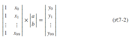
A = np.vstack([xi**0, xi**1])

$A^T$即式7-2的$100\times 2$的那个矩阵，代码里用的vstack函数在NumPy的数组合并与拆分一章有讲过。

3).调用scipy.linalg.lstsq传入$A^T$和观测值里的$y_i$即程序里的yi变量即可求得$f(x) = a + bx$里的a和b。a和b记录在lstsq函数的第一个返回值里。

sol, r, rank, s = la.lstsq(A.T, yi)

4). scipy.linalg.lstsq的第一个返回值sol共有两个值，sol[0]即是估计出来的$f(x) = a + bx$里a，sol[1]代表$f(x) = a + bx$里b。因此$f(x)$为：

y_fit = sol[0] + sol[1] * x

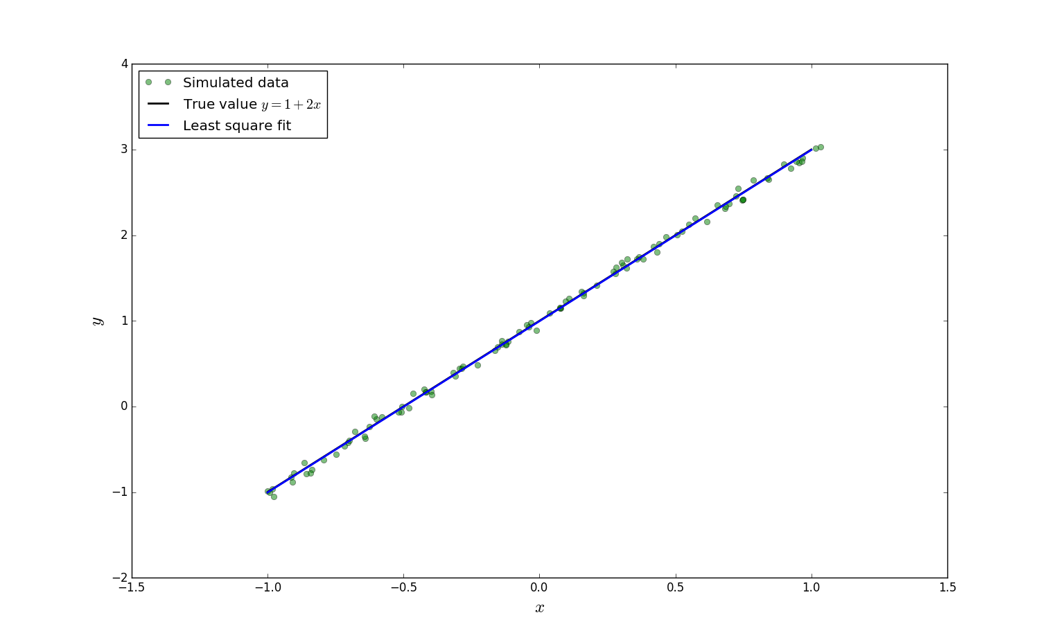
至此找到了这100个($x_i,y_i$)的模型方程。从print sol语句的输出结果可以看出数据还是比较接近$y = 2 x + 1$的。

完整程序如下：

import numpy
import scipy.linalg as la
import numpy as np
import matplotlib.pyplot as plt
m = 100
x = np.linspace(-1, 1, m)
y_exact = 1 + 2 * x
xi = x + np.random.normal(0, 0.05, 100)
yi = 1 + 2 * xi + np.random.normal(0, 0.05, 100)
print xi,"#xi"
print yi,"#yi"
A = np.vstack([xi**0, xi**1])
sol, r, rank, s = la.lstsq(A.T, yi)
y_fit = sol[0] + sol[1] * x 
print sol,r ,rank,s 
fig, ax = plt.subplots(figsize=(12, 4))
ax.plot(xi, yi, 'go', alpha=0.5, label='Simulated data')
ax.plot(x, y_exact, 'k', lw=2, label='True value $y = 1 + 2x$')
ax.plot(x, y_fit, 'b', lw=2, label='Least square fit')
ax.set_xlabel(r"$x$", fontsize=18)
ax.set_ylabel(r"$y$", fontsize=18)
ax.legend(loc=2)
plt.show()

可视化输出结果：如果看到此处没啥问题，恭喜您！您已经掌握明白了机器学习里的线性回归了。

7.2 再给一个例子

这个程序和7.1节的程序差不多，只不过模型变成了$f(x_i) = a + bx + cx^2$了而已，请自己分析分析。

import numpy
import scipy.linalg as la
import numpy as np
import matplotlib.pyplot as plt
x = np.linspace(-1, 1, 100)
a, b, c = 1, 2, 3
y_exact = a + b * x + c * x**2
m = 100
xi=1 - 2 * np.random.rand(m)
print "xi.shape", xi.shape,xi**1,xi
yi=a + b * xi + c * xi**2 + np.random.randn(m)
A = np.vstack([xi**0, xi**1, xi**2])
print A.shape, A.T.shape
sol, r, rank, s = la.lstsq(A.T, yi)
y_fit = sol[0] + sol[1] * x + sol[2] * x**2
fig, ax = plt.subplots(figsize=(12, 4))
ax.plot(xi, yi, 'go', alpha=0.5, label='Simulated data')
ax.plot(x, y_exact, 'k', lw=2, label='True value $y = 1 + 2x + 3x^2$')
ax.plot(x, y_fit, 'b', lw=2, label='Least square fit')
ax.set_xlabel(r"$x$", fontsize=18)
ax.set_ylabel(r"$y$", fontsize=18)
ax.legend(loc=2)
plt.show()

可视化输出结果：

7.3 总结

本章在解释最小二乘时$J(\theta)$用到了前边章节的范数的概念、通过最小二乘法实现了机器学习里的线性回归问题。